.png)
Table of contents
Data processing
About the data
Source: Kaggle - Hotel Booking
The dataset have 3 file:
-
The original, raw data set is given in the hotel_bookings.csv file.
-
bookings_2023.csv is a slightly simplified version with 23 features.
-
The bookings.csv file has been further reduced to 10 columns and pre-processed to aid analysis.
Since this is hotel real data, all data elements pertaining hotel or costumer identification were deleted.
The three datasets are essentially variations of one another, ‘hotel booking’ has been chosen as the primary dataset due to its raw data.
Data overview
Data has 119.390 rows and 32 columns.
| Number | Customers Source | Customer Character | Reservation | Recorded time |
|---|---|---|---|---|
| 1 | hotel | adults | is_canceled | arrival_date_year |
| 2 | market_segment | children | lead_time | arrival_date_month |
| 3 | distribution_channel | babies | days_in_waiting_list | arrival_date_week_number |
| 4 | agent | country | stays_in_weekend_nights | arrival_date_day_of_month |
| 5 | company | is_repeated_guest | stays_in_week_nights | reservation_status |
| 6 | customer_type | previous_cancellations | reserved_room_type | reservation_status_date |
| 7 | previous_bookings_not_canceled | assigned_room_type | ||
| 8 | booking_changes | |||
| 9 | deposit_type | |||
| 10 | adr | |||
| 11 | required_car_parking_spaces | |||
| 12 | meal | |||
| 13 | total_of_special_requests |
Data cleaning
Duplicated
Input
# checking total duplicated
hotel_booking.duplicated().sum()
31994
As authors claims that:
- “Each observation represents a hotel booking.”
and- “Since this is hotel real data, all data elements pertaining hotel or costumer identification were deleted.”
Cause of ‘Each observation represents a hotel booking’ therefore data record is separate customers from separate hotels and coincidencelly have the same data. the action here is choose to keep all the duplications.
Null and Undefined data
# checking null
hotel_booking.isnull().sum().sort_values(ascending=False)
company                           112593
agent                              16340
country                              488
children                               4
# check columns have that have 'Undefined' values
columns_with_value = (hotel_booking == 'Undefined')

columns_with_value.sum().sort_values(ascending=False)
meal                              1169
distribution_channel                 5
market_segment                       2
in short:
| columns | problem |
|---|---|
| agent | has nan |
| company | has nan |
| children | has nan |
| country | has nan |
| meal | has Undefined |
| market_segment | has Undefined |
| distribution_channel | has Undefined |
Author claim that:
In some categorical variables like Agent or Company, “NULL” is presented as one of the categories.
This should not be considered a missing value, but rather as “not applicable”.
For example, if a booking “Agent” is defined as “NULL” it means that the booking did not came from a travel agent.
As said above:
for the ‘agent’ and ‘company’ columns can change ‘nan values’ into:
- 0 as customer not come from agent/company
- 1 as customer come from agent/company
# create def to change data value
def convert_num(i):
    if i > 0:
        return 1
    return 0

# apply def
hotel_booking['agent_encode'] = hotel_booking.agent.apply(convert_num)
hotel_booking['company_encode'] = hotel_booking.company.apply(convert_num)

# 'children' columns has 4 nan values replace by median
hotel_booking['children'] = hotel_booking['children'].fillna(hotel_booking['children'].median())

# 'country' columns has 488 nulls values
# not using to run model but can use to illustrate customer character
# leave as it is
hotel_booking.country.isnull().sum()
hotel_booking.country.value_counts()
for the ‘Undefined’ values:
# as dictionary states that:
# - Undefined/SC : no meal package
# - BB : Bed & Breakfast
# - HB : Half board (breakfast and one other meal – usually dinner)
# - FB : Full board (breakfast, lunch and dinner)

# as said: encode 'meal' as Undefined/SC: 0 and others: 1
def convert_meal(j):
    if j == 'Undefined' or j == 'SC':
        return 0
    return 1

hotel_booking['meal_encode'] = hotel_booking.meal.apply(convert_meal)

# 'market_segment' and 'distribution_channel' have less than 6 'undefined' values
# leave as it is
print(hotel_booking.market_segment.value_counts())
print('-----------')
print(hotel_booking.distribution_channel.value_counts())
Outliers
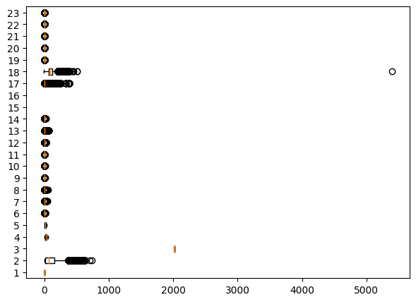
Showed that columns 18 which is ‘adr’ has 1 outliers -> choose to delete that row
# drop outliers
hotel_booking = hotel_booking[hotel_booking['adr'] < 1000] #.reset_index(drop=True, inplace=True)
Merge columns
Merge columns that have similar meaning
# create columns 'family_size' for illustation
hotel_booking['family_size'] = hotel_booking['adults'] + hotel_booking['children'] + hotel_booking['babies']

# booking_requests = booking_changes + required_car_parking_spaces + total_of_special_requests : cause of this is all request in booking process.
hotel_booking['booking_requests'] = hotel_booking.booking_changes + hotel_booking.required_car_parking_spaces + hotel_booking.total_of_special_requests

# stay_in_days = stays_in_weekend_nights + stays_in_week_nights
hotel_booking['stay_in_days'] = hotel_booking.stays_in_weekend_nights + hotel_booking.stays_in_week_nights
Create data for illustrate and calculate
# create columns 'source' for illustrate customer sources
hotel_booking['source'] = np.where((hotel_booking['agent'] > 0) & (hotel_booking['company'] > 0), 'both',
                          np.where(hotel_booking['agent'] > 0, 'agent',
                          np.where(hotel_booking['company'] > 0, 'comapny',
                          'not applicable')))

---

# create columns 'meal_request'
meal_dictionary = {'BB': 'Meal', 'FB': 'Meal', 'HB': 'Meal',
                   'SC': 'No meal', 'Undefined': 'No meal'}
hotel_booking['meal_request'] = hotel_booking['meal'].map(meal_dictionary)

---

# create columns 'repeated_guest'
repeated_guest_dictionary = {0: 'New guest', 1: 'Old guest'}
hotel_booking['repeated_guest'] = hotel_booking['is_repeated_guest'].map(repeated_guest_dictionary)

---

# create columns 'cancelation_status'
cancel_dictionary = {0: 'Check_in', 1: 'Canceled'}
hotel_booking['cancelation_status'] = hotel_booking['is_canceled'].map(cancel_dictionary)

---

# create columns 'total_booking'
hotel_booking['total_booking'] = hotel_booking.previous_cancellations + hotel_booking.previous_bookings_not_canceled + 1

---

# create columns 'total_cancelation'
hotel_booking['total_cancelation'] = hotel_booking['previous_cancellations'] + hotel_booking['is_canceled']

---

# create 'cancelation_rate'
hotel_booking['cancelation_rate'] = (hotel_booking['total_cancelation'] / hotel_booking['total_booking'] )* 100
Drop unnescessary columns
Drop columns below cause of:
- reservation_status: exactly as ‘is_canceled’ columns
- reservation_status_date: not see the use
- arrival_date_year: this analysis focus on customer behaviours in months and days
- arrival_date_week_number: this analysis focus on customer behaviours in months and days
- company: replace by ‘company_encode’
- agent: replace by ‘agent_encode’
- market_segment: similar with distribution_channel
- adults, children, babies: replace by ‘family size’
- stays_in_weekend_nights, stays_in_week_nights: replace by ‘stay_in_days’
hotel_booking = hotel_booking.drop(['reservation_status', 'reservation_status_date', 'arrival_date_year', 'arrival_date_week_number',
                                    'company', 'agent',
                                    'market_segment',
                                    'adults', 'children', 'babies',
                                    'booking_changes', 'required_car_parking_spaces', 'total_of_special_requests',
                                    'stays_in_weekend_nights', 'stays_in_week_nights'], axis=1)
EDA
- Overview:
# basic graphs
hotel_booking.hist(figsize= (20,20))
plt.show()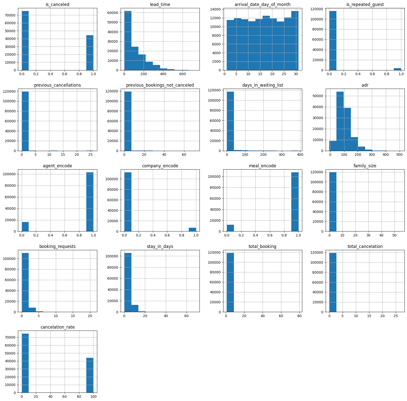
- Customer sources:
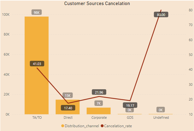
There are 5 distribution channels:
TA/TO: ‘TA’ mean ‘Travel Agents’ and ‘TO’ mean ‘Tour Operators’ and they are the main sources of customers with 82% (98,000 customers) booking by this channel. Cancelation rate of this channels take 41%.
Direct and Corporate have a relatively modest share, comprising just around 22.000 customers, less than half of TA/TO channel.
Other channels GDS (Global Distribution System) and Undefined have only 200 customers over 3 years of data.
Undefined customer has 100% cancelation rate.
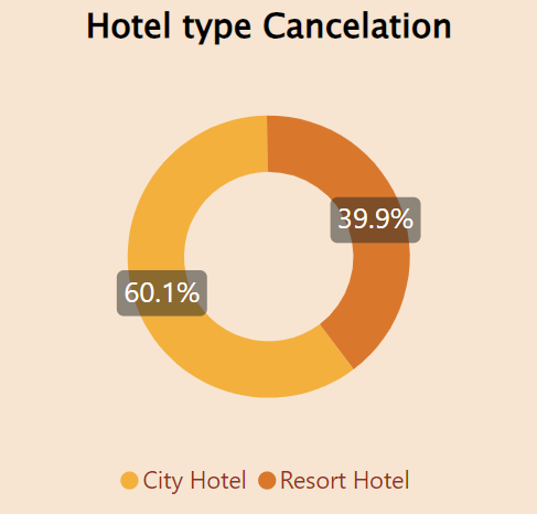
There are 2 types of hotel, City hotel and Resot hotel. Although 75% of bookings are for the City hotel, its cancellation rate is also high, standing at 60%.
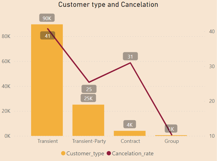
Transient customers is holding the high quantity of 90k customers, and their cancelation rate also the highest of 41%.
Only 577 customer from Group but their cancelation rate is only 10%.
Despite more than 4000 customers booking from the Contract being lower than the Transient-party, the Contract customer cancellation rate is 6% higher than that of the Transient-party.
- Customer character:
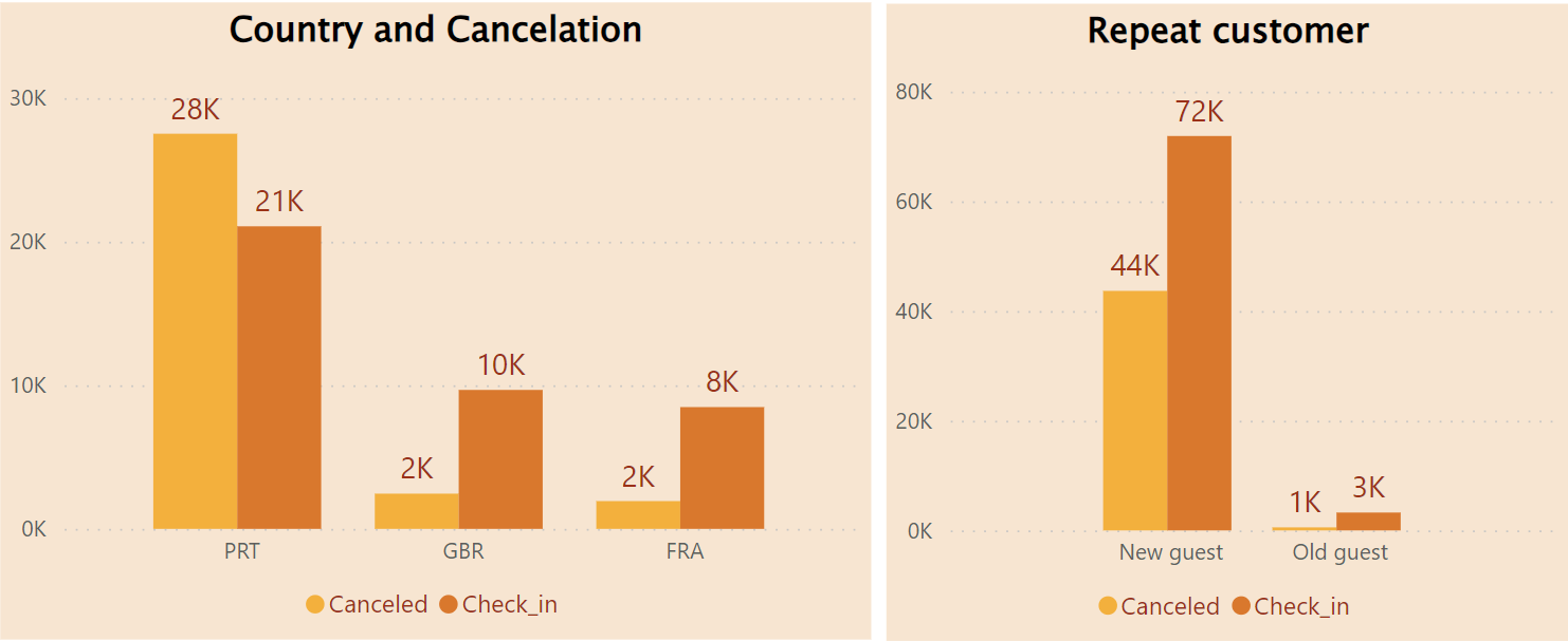
While most bookings come from Portuguese guests, their Cancellation is 1.3 times higher than their Check-in.
Other country have nearly half of the customers but their Cancelation is 4 to 5 times lower than their Check-in.
Booking by New-guests is 30 times higher than Old-guests. Cancelation in New guests is 37% but it is only 15% in Old guests.
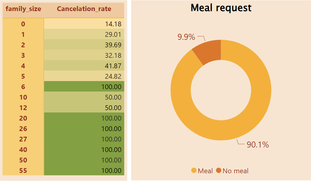
Family size from more 20 people and 6 people have absolute Cancelation rate. The lower the family size the lower Cancelation rate.
Only 10% booking not request meal.
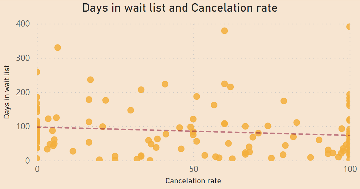
Waiting days can up to 400 days, but most booking comes around 200 days. There is no clear indication that waiting days relate to cancelation rate.
Machine learning process
Preparing
Encode
First, separate the numeric and categorical columns.
# seperate numeric columns
hb_numeric = hotel_booking.select_dtypes(include='number')
Then, encode the categorical columns, mostly using ‘onehot’
# encode the categories columns using onthot
hotel_dictionary = {'Resort Hotel': 1, 'City Hotel': 0}
hotel_booking['hotel_encode'] = hotel_booking.hotel.map(hotel_dictionary)

onehot_month            = pd.get_dummies(hotel_booking['arrival_date_month'], prefix = 'month').astype(int)
onehot_market           = pd.get_dummies(hotel_booking['distribution_channel'], prefix = 'market').astype(int)
onehot_reserved_room    = pd.get_dummies(hotel_booking['reserved_room_type'], prefix = 'reserved_room').astype(int)
onehot_assigned_room    = pd.get_dummies(hotel_booking['assigned_room_type'], prefix = 'assigned_room').astype(int)
onehot_deposit_type     = pd.get_dummies(hotel_booking['deposit_type'], prefix = 'deposit_type').astype(int)
onehot_customer_type    = pd.get_dummies(hotel_booking['customer_type'], prefix = 'customer_type').astype(int)
Finish by create new dataset.
# create new dataset to concate 2 datasets

hb_encode = pd.concat([
    hb_numeric, # the dataset
    onehot_month,
    onehot_market,
    onehot_reserved_room,
    onehot_assigned_room,
    onehot_deposit_type,
    onehot_customer_type
], axis = 1)
Defining X, y
First, to calculate correlation and draw a chart for a better view.
# calculate correlation of others columns to 'is_canceled'
hb_correlation = hb_encode.corr(numeric_only=True)[['is_canceled']]
hb_correlation.drop(index='is_canceled', inplace=True)
hb_correlation = hb_correlation.sort_values(by='is_canceled', ascending=False)

# plot chart
fig, ax = plt.subplots(figsize=(20, 20))

# draw a seperate linne at x = 0
ax.axvline(x=0, color='gray', linestyle='--')

# bar chart
colors = np.where(hb_correlation['is_canceled'] > 0, 'lightblue', 'lightcoral')
bars = ax.barh(hb_correlation.index, hb_correlation['is_canceled'], color=colors)

# rearrange value lable of bar chart
for bar in bars:
    width = bar.get_width()
    label_x_pos = width + 0.01 if width >= 0 else width - 0.05 # if value > 0 set in the right else set in the left
    ax.text(label_x_pos, bar.get_y() + bar.get_height() / 2, f'{width:.2f}', va='center', fontsize=13)

ax.set_xlabel('Correlation')
ax.set_title('Correlation with Cancelation', size=16)
plt.grid()
plt.tight_layout()
plt.show()
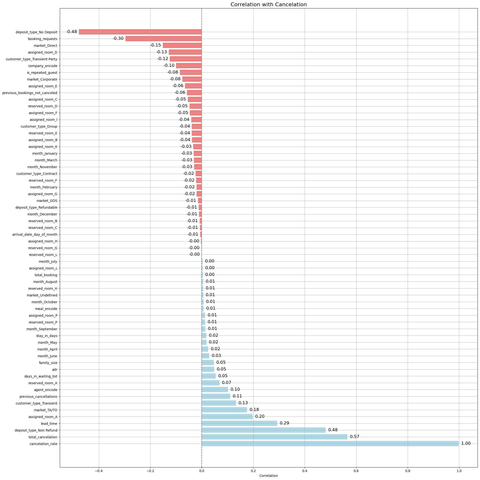
As showed in the graph:
‘cancelation_rate’ and ‘total_cancelation’ have high correlation with ‘is_canceled’ cause ‘is_canceled’ constitutes for their formular.
–> not use this columns in model to avoid false calculation.
Other than 2 above columns, overal correlation numbers are decent, no more than 0,5 and less than -0.5. Major of them are between -0,1 to 0,1. Therefore, those columns have correlation higher than 0,1 and lower than -0.1 are chosen.
# sort columns have value outside of this range (-0.1, 0.1)
sorted(hb_correlation[ ~hb_correlation['is_canceled'].between(-0.1, 0.1)].index)
['agent_encode',
 'assigned_room_A',
 'assigned_room_D',
 'booking_requests',
 'cancelation_rate',
 'customer_type_Transient',
 'customer_type_Transient-Party',
 'deposit_type_No Deposit',
 'deposit_type_Non Refund',
 'lead_time',
 'market_Direct',
 'market_TA/TO',
 'previous_cancellations',
 'total_cancelation']
Checking correlation of columns to each one another.
# create new dataset
hb_encode_corr =  hb_encode[['is_canceled',
                             'agent_encode',
                             'assigned_room_A',
                             'assigned_room_D',
                             'booking_requests',
                             'customer_type_Transient',
                             'customer_type_Transient-Party',
                             'deposit_type_No Deposit',
                             'deposit_type_Non Refund',
                             'lead_time',
                             'market_Direct',
                             'market_TA/TO',
                             'previous_cancellations'
                             ]]

# draw correlation heatmap

# create dataset correlation and only select the correlation out of the range (-0.1, 0.1)
def high_corr(value):
  if -0.2 < value < 0.2:
    return 0
  return value
hb_high_correlation = hb_encode_corr.corr(numeric_only=True)
hb_high_correlation = hb_high_correlation.applymap(high_corr)

# draw heatmap of correlation
plt.figure(figsize=(8,8))
sns.heatmap(hb_high_correlation, annot=True, cmap='RdYlGn', vmin=-1, vmax=1)
There are couples of columns that have high correlation with each other:
- customer_type_transient and customer_type_transient_party
- deposit_type_No_deposit and deposit_type_No_refund
- market_Direct and market_TA/TO
The choice is to delete 1 of each columns to prevent Multicollinearity (Đa cộng tuyến)
This is the chart after drop some of the above columns:
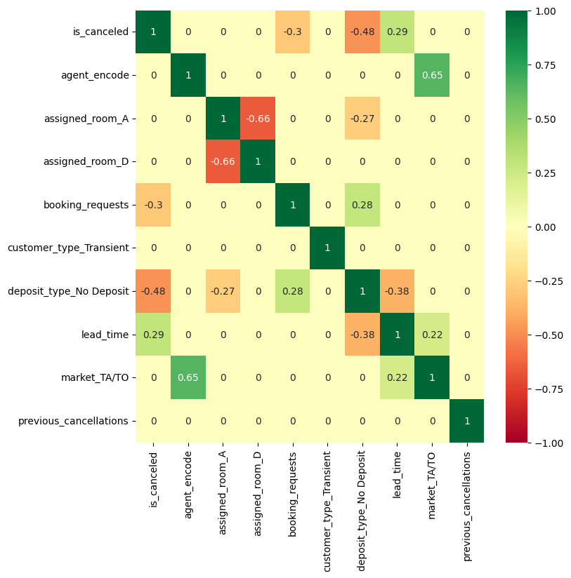
The X here is:
‘agent_encode’, ‘assigned_room_A’, ‘assigned_room_D’, ‘booking_requests’, ‘customer_type_Transient’, ‘deposit_type_No Deposit’, ‘lead_time’, ‘market_TA/TO’.
The y here is:
‘is_canceled’
Data balancing
hb_encode_corr['is_canceled'].hist()
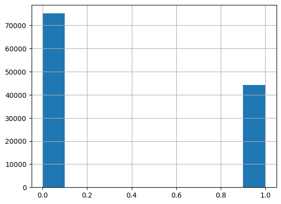
As showed that, the 0 values is double the 1 values, the choice here is to undersampling.
# dataset not cancel == 0
hbc_0 = hb_encode_corr[hb_encode_corr.is_canceled == 0]

# dataset is canceled == 1
hbc_1 = hb_encode_corr[hb_encode_corr.is_canceled == 1]

# dataset size
hbc_0.shape, hbc_1.shape
# random choose data from hbc_0
hbc_0_resapled = hbc_0.sample(44223, random_state=1)

# new dataset
hbc_0_resapled.shape
# connect hb_0 and hbc_1
hb_balance = pd.concat([hbc_0_resapled,hbc_1])

# y after rebalance
hb_balance['is_canceled'].value_counts()
is_canceled
0    44223
1    44223
Name: count, dtype: int64
Reset index for further use in normalization.
hb_balance.reset_index(drop=True, inplace=True)
Normalization: min-max scaler
# Scale X2
from sklearn.preprocessing import MinMaxScaler
scaler = MinMaxScaler()
X_scaled = scaler.fit_transform(hb_balance.iloc[:, 1:11].values)

# create new dataframe
hb = pd.DataFrame(data = X_scaled, columns = hb_balance.iloc[:, 1:11].columns)

# add y2 column
hb['is_canceled'] = hb_balance['is_canceled']
Split train-test dataset
# chose X, y

y = hb['is_canceled'].values
X = hb[['agent_encode', 'assigned_room_A', 'assigned_room_D', 'booking_requests', 'customer_type_Transient', 'deposit_type_No Deposit', 'lead_time', 'market_TA/TO']].values

# seting X_set for use
X_set = ['agent_encode', 'assigned_room_A', 'assigned_room_D', 'booking_requests', 'customer_type_Transient', 'deposit_type_No Deposit', 'lead_time', 'market_TA/TO']

# run split
from sklearn.model_selection import train_test_split

X_train, X_test, y_train, y_test = train_test_split(X, y, test_size=0.3, random_state=1)
Models
Logistic Regression
- Model setup
# import models
from sklearn.linear_model import LogisticRegression
model_logistic = LogisticRegression(random_state=1)
model_logistic.fit(X_train, y_train)
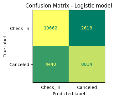
- Result
from sklearn.metrics import classification_report

# predict y
y_pred_logistic = model_logistic.predict(X_test)

# classification report
print(classification_report(y_test, y_pred_logistic))
              precision    recall  f1-score   support

           0       0.71      0.80      0.75     13280
           1       0.77      0.67      0.71     13254

    accuracy                           0.73     26534
   macro avg       0.74      0.73      0.73     26534
weighted avg       0.74      0.73      0.73     26534
- Add to dictionary to compare models
from sklearn.metrics import roc_auc_score
from sklearn.metrics import roc_curve

# confusion matrix
cnf_matrix = confusion_matrix(y_test, y_pred_logistic)
tn, fp, fn, tp = cnf_matrix.ravel()

# calculate probability and ROC_AUC_score
y1_proba_logistic = model_logistic.predict_proba(X_test)[:, -1]
false_positive_rate, true_positive_rate, threshold = roc_curve(y_test, y1_proba_logistic)
auc_score = roc_auc_score(y_test, y1_proba_logistic)

# class_report
report = classification_report(y_test, y_pred_logistic, output_dict=True)

# update dictionary to compare
model_results = {}
model_results['Logistic Regresson'] = {
  'Params': None,
  'TP': tp,
  'FN': fn,
  'TN': tn,
  'FP': fp,
  'FP_rate': false_positive_rate,
  'TP_rate': true_positive_rate,
  'ROC AUC Score': auc_score,
  'Precision':  report['1']['precision'],
  'Recall':     report['1']['recall'],
  'F1_Score':   report['1']['f1-score'],
  'Accuracy Score': report['accuracy'],
}
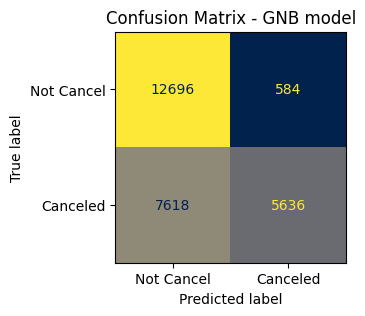
Gaussian Navie Bayes
- Model setup
from sklearn.naive_bayes import GaussianNB
model_GNB = GaussianNB()
model_GNB.fit(X_train, y_train)
- Result
# predict
y_pred_GNB = model_GNB.predict(X_test)

# classification report
print(classification_report(y_test, y_pred_GNB))
              precision    recall  f1-score   support

           0       0.62      0.96      0.76     13280
           1       0.91      0.43      0.58     13254

    accuracy                           0.69     26534
   macro avg       0.77      0.69      0.67     26534
weighted avg       0.77      0.69      0.67     26534
- Add to score dictionary
# confusion matrix
cnf_matrix = confusion_matrix(y_test, y_pred_GNB)
tn, fp, fn, tp = cnf_matrix.ravel()

# calculate probability and ROC_AUC_score
y_proba_GNB = model_GNB.predict_proba(X_test)[:, -1]
false_positive_rate, true_positive_rate, threshold = roc_curve(y_test, y_proba_GNB)
auc_score = roc_auc_score(y_test, y_proba_GNB)

# class_report
report = classification_report(y_test, y_pred_GNB, output_dict=True)

# update dictionary to compare
model_results['GNB'] = {
  'Params': None,
  'TP': tn,
  'FN': fp,
  'TN': fn,
  'FP': tp,
  'FP_rate': false_positive_rate,
  'TP_rate': true_positive_rate,
  'ROC AUC Score': auc_score,
  'Precision':  report['1']['precision'],
  'Recall':     report['1']['recall'],
  'F1_Score':   report['1']['f1-score'],
  'Accuracy Score': report['accuracy'],
}
Decision Tree
- Model setup: Finding max_depth
from sklearn import tree

# setup to find max_depth
tree_scores = []
for d in range(1, 21):
    model_tree = tree.DecisionTreeClassifier(max_depth=d, random_state=0)
    model_tree.fit(X_train, y_train)
    model_score = model_tree.score(X_test, y_test)
    tree_scores.append(model_score*100)

# Plot score
max_depth = [n for n in range(1, 21)]
max_n =     [n      for n, score in zip(max_depth, tree_scores) if score == max(tree_scores)]
max_score = [score  for n, score in zip(max_depth, tree_scores) if score == max(tree_scores)]
x_ticks =   [n      for n, score in zip(max_depth, tree_scores) if score == max(tree_scores)]

print(f"Mô hình có score cao nhất = {max_score[0]:.2f}% tại số tầng = {max_n}")

plt.figure(figsize=(10, 4))
plt.scatter(max_n, max_score, color='red', marker = 'o')
plt.plot(max_depth, tree_scores)
plt.ylabel('Accuracy (%)',fontsize=12)
plt.xlabel('max_depth',fontsize=12)
plt.xticks(x_ticks, size=10)
plt.title("Accuracy of Decision Tree by max_depth", size=16)
plt.grid()
plt.show()
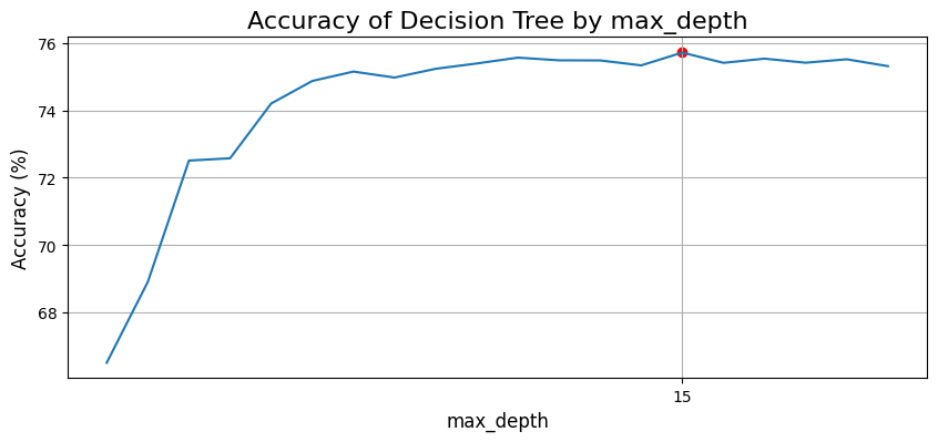
model_tree = tree.DecisionTreeClassifier(max_depth=15, random_state=1)
model_tree.fit(X_train, y_train)
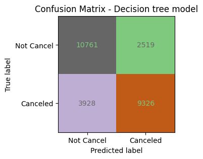
- Result
# predict
y_pred_tree = model_tree.predict(X_test)

# class_report
print(classification_report(y_test, y_pred_tree))
              precision    recall  f1-score   support

           0       0.73      0.81      0.77     13280
           1       0.79      0.70      0.74     13254

    accuracy                           0.76     26534
   macro avg       0.76      0.76      0.76     26534
weighted avg       0.76      0.76      0.76     26534
- Add to score dictionary
# confusion matrix
cnf_matrix = confusion_matrix(y_test, y_pred_tree)
tn, fp, fn, tp = cnf_matrix.ravel()

# calculate probability and ROC_AUC_score
y_proba_tree = model_tree.predict_proba(X_test)[:, -1]
false_positive_rate, true_positive_rate, threshold = roc_curve(y_test, y_proba_tree)
auc_score = roc_auc_score(y_test, y_proba_tree)

# class_report
report = classification_report(y_test, y_pred_tree, output_dict=True)

# update dictionary to compare
model_results['Decesion Tree'] = {
  'Params': 'max_depth = 1',
  'TP': tn,
  'FN': fp,
  'TN': fn,
  'FP': tp,
  'Precision':  report['1']['precision'],
  'Recall':     report['1']['recall'],
  'F1_Score':   report['1']['f1-score'],
  'Accuracy Score': report['accuracy'],
  'ROC AUC Score': auc_score,
  'FP_rate': false_positive_rate,
  'TP_rate': true_positive_rate,
}
Random Forest
- Model setup: Finding n_estimators
from sklearn.ensemble import RandomForestClassifier
rf_scores = []
for trees in range(70, 101):
    model_forest = RandomForestClassifier(n_estimators=trees, random_state = 1)
    model_forest.fit(X_train, y_train)
    model_score = model_forest.score(X_test, y_test)
    rf_scores.append(model_score)

# Plot score
n_estimators = [n for n in range(70, 101)]
max_n        = [n for n, score in zip(n_estimators, rf_scores) if score == max(rf_scores)]
max_score    = [score for n, score in zip(n_estimators, rf_scores) if score == max(rf_scores)]
x_ticks      = [n for n, score in zip(n_estimators, rf_scores) if score == max(rf_scores)]

print(f"Mô hình có score cao nhất = {max_score[0]:.2f} tại số cây = {max_n}")

plt.figure(figsize=(7, 2))
plt.scatter(max_n, max_score, color='red', marker = 'o')
plt.plot(n_estimators, rf_scores)
plt.xlabel('n_estimators')
plt.ylabel('Model Score')
plt.xticks(x_ticks, rotation=90, size=8)
plt.grid()
plt.show()
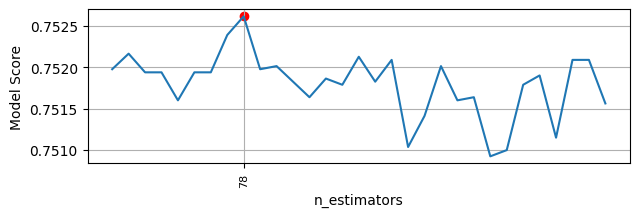
model_forest = RandomForestClassifier(n_estimators=99, random_state = 1)
model_forest.fit(X_train, y_train)
- Result
# predict
y_pred_forest = model_forest.predict(X_test)

# class_report
print(classification_report(y_test, y_pred_forest, digits = 4))
              precision    recall  f1-score   support

           0     0.7475    0.7622    0.7548     13280
           1     0.7569    0.7420    0.7494     13254

    accuracy                         0.7521     26534
   macro avg     0.7522    0.7521    0.7521     26534
weighted avg     0.7522    0.7521    0.7521     26534
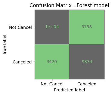
- Add to score dictionary
# confusion matrix
cnf_matrix = confusion_matrix(y_test, y_pred_forest)
tn, fp, fn, tp = cnf_matrix.ravel()

# calculate probability and ROC_AUC_score
y_proba_forest = model_forest.predict_proba(X_test)[:, -1]
false_positive_rate, true_positive_rate, threshold = roc_curve(y_test, y_proba_forest)
auc_score = roc_auc_score(y_test, y_proba_forest)

# class_report
report = classification_report(y_test, y_pred_forest, output_dict=True)

# update dictionary to compare
model_results['Random forest'] = {
  'Params': 'n_estimators = 90',
  'TP': tn,
  'FN': fp,
  'TN': fn,
  'FP': tp,
  'Precision':  report['1']['precision'],
  'Recall':     report['1']['recall'],
  'F1_Score':   report['1']['f1-score'],
  'Accuracy Score': report['accuracy'],
  'ROC AUC Score': auc_score,
  'FP_rate': false_positive_rate,
  'TP_rate': true_positive_rate,
}
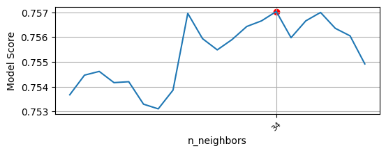
K Nearest Neighbor
- Model setup: Finding n_neighbor
from sklearn.neighbors import KNeighborsClassifier
knn_scores = []
for k in range(20, 41):
    model = KNeighborsClassifier(n_neighbors=k)
    model.fit(X_train, y_train)
    model_score = model.score(X_test, y_test)
    knn_scores.append(model_score)

# Plot score
n_neighbors = [k for k in range(20, 41)]
max_n =     [k      for k, score in zip(n_neighbors, knn_scores) if score == max(knn_scores)]
max_score = [score  for k, score in zip(n_neighbors, knn_scores) if score == max(knn_scores)]
x_ticks =   [k      for k, score in zip(n_neighbors, knn_scores) if score == max(knn_scores)]
print(f"Mô hình có score cao nhất = {max_score[0]:.2f} tại số cây = {max_n}")

plt.figure(figsize=(6, 2))
plt.scatter(max_n, max_score, color='red', marker = 'o')
plt.plot(n_neighbors, knn_scores)
plt.xlabel('n_neighbors')
plt.ylabel('Model Score')
plt.xticks(x_ticks, rotation=45, size=8)
plt.grid()
plt.show()

# n_neighbors = 34
from sklearn.neighbors import KNeighborsClassifier
model_KNN = KNeighborsClassifier(n_neighbors=34)
model_KNN.fit(X_train, y_train)
- Result
# predict
y_pred_KNN = model_KNN.predict(X_test)

# class_report
print(classification_report(y_test, y_pred_KNN, digits = 4))
              precision    recall  f1-score   support

           0     0.7344    0.8061    0.7686     13280
           1     0.7846    0.7079    0.7443     13254

    accuracy                         0.7570     26534
   macro avg     0.7595    0.7570    0.7564     26534
weighted avg     0.7595    0.7570    0.7564     26534
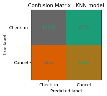
- Add to score dictionary
# confusion matrix
cnf_matrix = confusion_matrix(y_test, y_pred_KNN)
tn, fp, fn, tp = cnf_matrix.ravel()

# calculate probability and ROC_AUC_score
y_proba_KNN = model_KNN.predict_proba(X_test)[:, -1]
false_positive_rate, true_positive_rate, threshold = roc_curve(y_test, y_proba_KNN)
auc_score = roc_auc_score(y_test, y_proba_KNN)

# class_report
report = classification_report(y_test, y_pred_KNN, output_dict=True)

# update dictionary to compare
model_results['KNN'] = {
  'Params': 'n_neighbors = 1',
  'TP': tn,
  'FN': fp,
  'TN': fn,
  'FP': tp,
  'Precision':  report['1']['precision'],
  'Recall':     report['1']['recall'],
  'F1_Score':   report['1']['f1-score'],
  'Accuracy Score': report['accuracy'],
  'ROC AUC Score': auc_score,
  'FP_rate': false_positive_rate,
  'TP_rate': true_positive_rate,
}
Compare models
# combine and set dataframe
model_results_df = pd.DataFrame.from_dict(model_results, orient='index').reset_index()
model_results_df.rename(columns={'index':'model'}, inplace=True)
model_results_df

# create ROC chart
models = model_results_df['model'].unique()
colors = ['tab:blue','tab:orange','tab:green','tab:red','tab:purple','tab:gray']

plt.figure(figsize=(10,5))

# ROC curve
for model, color in zip(models, colors):
  plt.plot( model_results[model]['FP_rate'] ,model_results[model]['TP_rate'], linewidth=2, color=color )
plt.legend(['Logistic Regression', 'Gaussian Naive Bayes', 'Decision Tree', 'Random Forest', 'K Nearest Neighbors', 'Support Vector Machine'], fontsize=12)

# Random chances line
plt.plot([0,1], ls='--', linewidth=1, color='black')

# set lable
plt.xlabel('False Positive Rate', fontsize=16)
plt.ylabel('True Positive Rate', fontsize=16)

# title
plt.title('ROC curves', fontsize=16)

plt.plot()
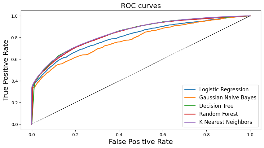
Showed in the chart that Logistic and Gaussian Naive Bayes have lower lines than other models.
# compare accuracy chart
plt.figure(figsize=(5, 2))
bars = plt.barh(model_results_df['model'], model_results_df['Accuracy Score'], color=colors)

# add % accuracy
for bar, acc_score in zip(bars, model_results_df['Accuracy Score']):
    plt.text(bar.get_width() + 0.02, bar.get_y() + bar.get_height() / 2, f'{acc_score*100:.2f}%', va='center')

plt.title('Accuracy Score', fontsize=13)

# set ticks
plt.xlim(0, 1)
plt.xticks([0, 0.2, 0.4, 0.6, 0.8, 1], ['0%', '20%', '40%', '60%', '80%', '100%'])

plt.show()
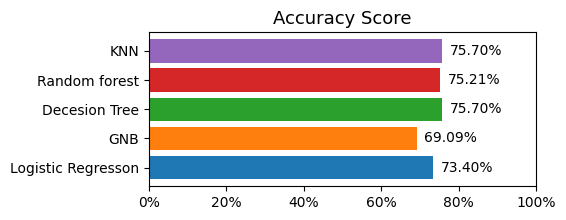
Accuracy score of most model is around 69% to 75%, and the lowest is Gaussian Naive Bayes. The highest is KNN and Decision Tree with 75.70%
# compare AUC chart
plt.figure(figsize=(5, 2))
bars = plt.barh(model_results_df['model'], model_results_df['ROC AUC Score'], color=colors)

# add % AUC
for bar, auc_score in zip(bars, model_results_df['ROC AUC Score']):
    plt.text(bar.get_width() + 0.02, bar.get_y() + bar.get_height() / 2, f'{auc_score*100:.2f}%', va='center', fontsize=12)

plt.title('ROC AUC Score', fontsize=13)

# set ticks
plt.xlim(0, 1)
plt.xticks([0, 0.2, 0.4, 0.6, 0.8, 1], ['0%', '20%', '40%', '60%', '80%', '100%'])

plt.show()
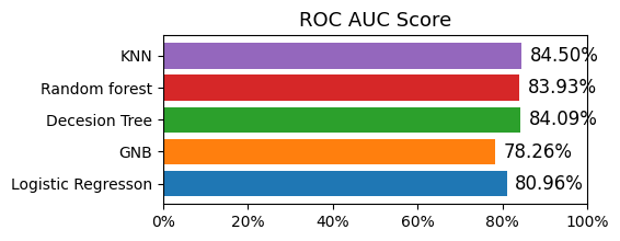
ROC AUC score has average of 80%, highest is KNN with 84.50% and lowest is GNB 78.26%.
For the conclusion, the model have the best performance is KNN, second model is Decision Tree.
Should not use GNB for this data.
Author: Thi Phong